How to Create a Data Validation Form

When inputting data into a spreadsheet, often you will find yourself having to type the same data into cells. That's where Data Validation comes in handy. Instead of typing the same thing over and over again, you can turn the cells into drop-down lists. That way, you could just quickly select an item from the list and move on to the next entry.
For example, suppose you had a column heading called "Student Grade". Even though there are only two grades available, Pass and More Work Needed, it can become quite laborious having to type either one or the other. Spelling mistakes will become increasingly more likely the more times you have to enter the grades. Much better to have a drop down list where you could select the grade. And no more spelling mistakes!

Data Validation

We'll now construct a spreadsheet with drop-down lists. The one we're going to construct takes us back to the classroom and our students from previous section.
So start a new spreadsheet, and format it to match the one below:

Before we can turn the cells in an entire column into drop down lists, we need some data to go in the lists. So starting at cell F2, add the following to your spreadsheet:

The data in columns F, G and H will be going into our lists. We can then hide this data so that it's not messing up our spreadsheet. You'll see how to do this later. But we can now turn Columns A, B and C into lists.

To turn the cells in an entire Column into a list, do the following:

• Highlight the whole of Column A by clicking on the letter A at the top of the column
• With the whole of Column A highlighted, click on Data from the Excel menu bar
• From the drop down menu, click Validation
• The following dialogue box appears:
  

• Make sure the Settings tab strip is selected
• Click the black down arrow just to the right of “Allow: Any Value”
• A drop down list appears
• Choose List
• A Source box appears on the dialogue box

The Source is the data that is going into your list. So you need to select the cells with the students in them. To select the cells with the students in them, do this:

• Click on the icon to the right of the Source text box:

• When you click the icon, the dialogue box contracts
• Click inside cell F2 on your spreadsheet
• Hold down your left mouse button, and drag to cell F9
• Then click on the icon again to expand the dialogue box
• The images below show the highlighting and expanded process in action

Click the icon and highlight F2 to F9

Click the icon again to expand the dialogue box

• If you have done it all correctly, your dialogue box will now look like this one:

So the Validation criteria should be: "Allow List", and the Source should be = $F$2:$F$9.

Click OK when your dialogue box reads the same as the one above. The cells in you entire A column will now be drop down lists. Test it out. Click on cell A3, for example. It should look like this:

If you click the black down arrow, you should see your list of students. Like the one below:

Click on any student in the list. The student appears in cell A3. Click on another cell in column A and try it again.

I'm sure you'll agree that it's much better than having to type out a student's name over and over again.

Except we have a slight problem. If you click inside cell A1 you'll see that this too has a drop down list. Clearly we don't want this to happen for our heading. To turn off the list in cell A1, do the following:

• Click inside cell A1
• From the Excel menu bar, click on Data
• From the drop down menu, click Validation
• From the Settings tab strip of the dialogue box, change "Allow List" to "Allow Any Value"
• Click OK

Time for you to try it alone. Change the Subject and Grade columns into drop down list, and then turn off the list for the headings cells B1 and C1.
The drop down lists for the Subject and Grade columns should look like these when you're done:

In the next part, you'll learn how to display error messages. That way, you can control what data your users are allowed to enter.

Data Input Forms

Computer Tutorials List Beginners Computing Word 2007 to 2010 Word 2000 to 2003 Excel 2007 to 2010 > Excel 2000 to 2003 < Web Design Cascading Style Sheets Javascript Visual Basic .NET Beginners PHP C# .NET Java for Beginners Qualifications and Certificates

How to Create a Data Input Form in Microsoft Excel Forms help you input data into a spreadsheet more easily. We'll look at a data input form. We're going to see how helpful a data input form is, and how easy it is to create one. In fact, you won't be creating one at all - Excel does all the work for you. First, the problem. Data Input Forms Start a new spreadsheet. Enter January in cell A1. AutoFill the months up to October in column J. Then do the following: Highlight the entire A column by clicking on the letter A at the top of the spreadsheet Hold down your left mouse button on the letter A of the column Keep it held down and drag to the right Keep dragging until you have highlighted all the columns from A to J Your highlighted spreadsheet will look like this: Once you have the columns A to J highlighted, click on Format from the menu bar From the drop down menu, select Column. A sub menu appears From the sub menu, click on Width The following little dialogue box pops up: Change your Column width to 15 and then click OK What should happen is that columns H to J disappear from the screen, and you can no longer see August to October. Now enter a number for each month. Any number will do. What happened? You should find yourself having to scroll across the spreadsheet in order to enter number for the months not on the screen. When you got to October, only the months May to October are visible. If you want to enter some more numbers, starting with January again, you have to scroll back to the start. Clearly this is a problem, if you have lots of data to enter. You don't really want to be scrolling backwards and forwards. Especially if you had over a hundred rows to fill. It would drive you nuts! There is an easier way - use a Form for the data inputting. To see how much more simple your life would be, do the following: Click inside cell A3 of your spreadsheet From the Excel menu bar, click on Data From the drop down list, click Form A form like the one below should pop up on top of your spreadsheet: As you can see, the labels for the months are on the left. To the right of each month there is a text box. The numbers currently in them are the numbers inputted on the spreadsheet. Click the New button at the top The text boxes go blank Click inside the January text box and enter a new number Enter new number for the rest of the months When you have finished, click the New button again When you click the New button, Excel will enter the numbers into your spreadsheet. The text boxes will be blanked out, ready for some new data. And that's it. No more scrolling! Easy, hey? The form even gives you button to set up some search criteria (Find and Criteria buttons). When you want to get back to your spreadsheet, just click the Close button.

Microsoft Excel 2007 to 2010

Insert Drawing Objects into your Excel Spreadsheets

A drawing can liven up a dull spreadsheet. Some good line art, or even simple shapes, can help illustrate your data. In this lesson, you'll see how to add simple shapes, and textboxes to your spreadsheet.

First, look at the spreadsheet below. Unless you know about Cosines, Adjacent angles, and Hypotenuse, the data below will be a bit bewildering:

However, add a few shapes, along with some colour, and it becomes clearer what the data is for (the Cosine in the image below has been formatted to 2 decimal places):

We'll now show you how to produce a spreadsheet like the one above. Don't worry if you haven't a clue about Cosines - it's not important for this lesson. (We'll show you the formula, though.)

How to Draw a Shape on an Excel Spreadsheet

To insert a shape on your spreadsheet, do the following.

• From the Excel Ribbon, click on Insert
• Locate the Shapes panel:

On the Shapes panel, click the drop down arrow to see all the available shapes:

• Under Basic Shapes, select the Right Triangle
• Hold down your left mouse button on your spreadsheet, and drag to create your shape. Let go when you have a decent sized triangle. You'll see something like this:

The green circle allows you to rotate the shape. The other circles (and squares) are sizing handles. Hold your mouse down over one of these and drag to resize your shape, if it's not the size you want it.

But we'd like the triangle pointing the other way. So hold your mouse down on the green circle, and drag to rotate your triangle:

You should see an outline, like the one above. Let go of your left mouse button when it is in position:

As you can see, the green circle is now on the left hand side.

If you look on the Excel Ribbon at the top, you'll notice that it has changed - a Format tab has appeared. You'll see all the various options for shapes. Locate Shape Fill on the Shape Styles panel, and click to see the Fill options:

Select a colour for your triangle. You'll also want to select a Shape Outline, underneath Shape Fill. Select the same colour as your Fill, and your triangle will look something like this one:

Add a Text Box to an Excel Spreadsheet

To get the letter B in the triangle, we'll add a text box. So, on the Insert Shapes panel again, you'll notice a Text Box option. Click on this to select it:

Now move back to your spreadsheet, hold down your left mouse button, and drag out a Text Box. Let go of the left mouse button and you'll have something like this:

With the cursor inside of the Text Box, simply type the letter B. Because it's text, you can highlight your letter and format it. In the image below, we've increased the font size:

We now need to drag our Text Box onto the shape. Move your mouse over the Text Box until the cursor changes shape to four arrowheads (this can be tricky):

Once your cursor changes shape, hold down the left mouse button and drag your Text Box on to the triangle:

With the Text Box selected, use the arrow keys on your keyboard to nudge it in to position. Fill the Text Box in the same way as you did for the triangle. It will then look like this:

If you need to move your triangle and Text Box, you can select them both at the same time, and drag them as one. Click on your Triangle to select it. Now hold down the CTRL key on your keyboard. With the CTRL key held down, click on your Text Box. Both will now be selected:

With both the triangle and the Text Box selected, hold your mouse over the selected shapes. When your cursor changes to the four arrowheads, hold down the left button and drag your shapes to a new position:

You can finish off the formatting in the normal way. In the image below, we selected all the cells surrounding the shape, and added a background colour from the Home menu, Font panel.

If you look again at the finished version, you'll see the rest of the colours we chose. These are just filled cells from the Home > Font panel:

The text in the cells is just entered in the normal way. The formula for the Cosine in cell G22 of our spreadsheet has this syntax:

=DEGREES(COS(Adjacent_Cell_Reference / Hypotenuse_ Cell_Reference))

An example of how to use is it this:

=DEGREES(COS(F18 / F10))

When the user types in a value for the Hypotenuse or the Adjacent, the Cosine number will change.
But you can add any shapes you want to liven up your spreadsheet. It doesn't have to look plain, white and dull!

And that completes this beginners course on Excel 2007 and Excel 2010. It may have a little taxing along the way, but if you've finished all of it, you should have quite a few new skills to show off!

Microsoft Excel 2007 to 2010

How to reference formulas and data on other worksheets

You don't have to have all your data on one worksheet. In fact, it's common practise to create lots of worksheets in the same workbook. In this lesson, you'll see how reference a formula that is on a different worksheet. This comes in handy if, for example, you have 12 worksheets, one for each month of the year. You can then create another worksheet that holds things like totals for the entire year. We'll do that now.

• Open up Excel (If it's already open, close the project you're currently working on and open a new blank workbook.)
• Locate Sheet1, Sheet2, and Sheet3 at the bottom of Excel
• Rename these to May, June, July (Right click, and select Rename from the menu)

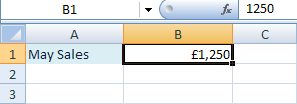
Click on the May sheet, and enter the same data as in the following image:

Click on the June sheet and enter the following:

Then click on the July sheet and enter the following:

We now need to create a new worksheet. So click on the New Worksheet icon at the bottom of Excel (the one to the right of July in the image below):

This will be called Sheet4 by default. Rename it to Annual Total, and your workbook will look like this at the bottom:

We're now going to add up the figures on the May, June and July worksheets, and put the answer on the Annual Total worksheet.

Add a label to your Annual Total worksheet:

Then click inside cell B1.

To reference data on another worksheet, you use the exclamation mark (exclamation point, if you're in the USA). This is commonly called a Bang!
So enter this in cell B1 of your Annual Total worksheet:

=May!B1

So we start with an equals sign (=), and then type the Name of the worksheet we want to reference (May). After the exclamation mark (bang), we have the cell we want to reference (B1). If you just type B1 by itself, Excel would assume that you meant the current worksheet.
When you press the enter key, you should see this on your Annual Total worksheet:

This is the same figure as the one on your May worksheet. To add up all our monthly worksheets, just reference them in the same manner:

=May!B1 + June!B1 + July!B1

So click inside cell B1 of your Annual Total worksheet and replace your formula with the one above. Press the enter key and you should see the answer:

So when you want to include figures or formula from other worksheets, remember to include the name of the worksheet followed by a bang

In the next part, you'll see how to spruce up an Excel spreadsheet with drawing objects.

Microsoft Excel 2007 to 2010

Object Linking and Embedding

Object Linking and Embedding (or OLE for short) is a technique used to insert data from one programme into another. We'll create a simple spreadsheet to illustrate the process, and place it in to Word document. When the Excel spreadsheet is updated, you'll see the Word version update itself as well.

If you don't want the data to update in Word, for example, it's called Embedding; if you do want the data to update, it's called Linking. We're going to do Linking. For this exercise, you need Word 2007 as well as Excel 2007 (or both 2010 versions).
First, create the simple spreadsheet below, and enter the formula shown in cell E3:

When you enter a number in cell E1, the answer is placed in cell E3 (don't do this yet).

With your spreadsheet created, highlight the cells A1 to E3. Click on the Home tab in Excel. On the Clipboard panel, click on Copy.
Now switch to Word 2007/2010. On the Home tab in Word 2007/2010, locate the Clipboard panel, and the Paste item:

Click on Paste. From the Paste menu, select Paste Special:

When you click on Paste Special, you'll see the following dialogue box appear:

Select Microsoft Office Excel Worksheet Object from the dialogue box. On the left hand side, select Paste Link. Click OK.

When you click OK, Word 2007/2010 will insert the spreadsheet from Excel:

It's even retained the cell formatting!

To check that it really does update in Word 2007/2010, switch back to Excel. Click inside Cell E1 and enter the number 7. Press the Enter key on your keyboard, and you should have the same answer as in the image below:

Now switch back to Word 2007/2010, and you should see that it too has the same answer:

Word 2007/2010 has successfully linked the data from Excel 2007/2010! If you don't want the updates, you would choose Paste from the Paste Special dialogue box instead of Paste Link.

You can link or embed things like Charts or Pivot Tables into Word 2007/2010, though, and it can come in really useful.

In the next part, you'll see how to reference formulas and data on other worksheets.